The Application of Hidden Markov Moodel to Detect BTC Makret Regime

Project description

• Language: Python
• Libraries: hmmlearn, numpy, pandas, sklearn
• Project type: Quant trading research, market regime learning
• Data source: Binance BTCUSDT OHLCV candles (pre-collected in multiple timeframes)

In this research note, I share my ongoing work on applying Hidden Markov Models (HMM) to BTC market regime detection. The objective is not to predict exact future prices, but to infer latent market states (regimes) and study how those states persist and transition over time.

Binance integration in this project is straightforward: BTCUSDT candles are collected and stored in parquet format, then used as time-series input for regime learning.

Hidden Markov Model: Theoretical Foundation

An HMM assumes that observed data is generated by an unobserved (hidden) state process.

1. Hidden state at time t: z_t in {1, 2, …, K}
2. Markov property: P(z_t | z_{t-1}, z_{t-2}, …) = P(z_t | z_{t-1})
3. Transition matrix: A_{ij} = P(z_t = j | z_{t-1} = i)
4. Emission model: observations x_t are sampled from a distribution conditioned on z_t

For financial regime modeling, this means:

• The market can be in one latent regime at each time step.
• Regimes switch probabilistically.
• Returns, volatility, and volume patterns are regime-dependent.

The Hierarchical Nature of HMM

The model is hierarchical in three levels:

1. Regime dynamics layer A latent Markov chain controls regime switching through the transition matrix.

2. State-specific distribution layer Each regime has its own emission distribution parameters.

3. Observed feature layer The actual market features (returns, volatility, volume behavior) are emitted from the active regime.

This hierarchy is useful because it separates structural market behavior (state transitions) from noisy short-term observations (feature realizations).

Why Gaussian Mixture HMM (GMM-HMM)

The proposed model uses GMM-HMM, not a single-Gaussian HMM.

self.model = hmm.GMMHMM(
    n_components=4,
    n_mix=4,
    covariance_type="diag",
    n_iter=100,
    tol=1e-4
)

The reason is distributional: crypto returns are often heavy-tailed and asymmetric. A single Gaussian per state is usually too restrictive. A mixture of Gaussians lets each regime represent:

• central/normal behavior
• tail behavior (extreme moves)

This improves flexibility without abandoning probabilistic structure.

Alternatives and Why They Were Not the Main Choice

Several alternatives were considered:

1. GaussianHMM (single Gaussian per state) Simpler and faster, but weaker under fat tails.

2. Markov-Switching AR / econometric regime models Strong for some macro-style datasets, but less flexible with multivariate emission features.

3. Student-t based state-space variants Potentially better tail modeling, but more complex implementation pipeline.

4. Non-temporal clustering (k-means, GMM without Markov chain) Can cluster observations, but cannot model regime persistence and transition dynamics.

Given this trade-off, GMM-HMM is a good balance of interpretability, temporal structure, and fat-tail tolerance.

Feature Set and Financial Reasoning

The feature set is chosen to represent direction, uncertainty, and participation:

1. Log returns Primary direction signal for bullish/bearish separation.

2. Fractionally differenced returns A compromise between stationarity and memory preservation.

3. Log volatility (high/low range) Captures turbulence and intraperiod risk.

4. Log volume change Tracks participation shocks, often relevant near regime shifts.

5. Rolling mean and rolling std of returns Stabilize short-run noise and reduce unstable regime flipping.

So, the HMM does not observe price level directly as regime identity. It observes behavior statistics that are more regime-informative.

Regime Findings from the Current Run

The current 4-state run learns directional-volatility regimes such as:

• Trend Up (Low Vol)
• Trend Up (High Vol)
• Trend Down (Low Vol)
• Trend Down (High Vol)

State persistence is high (self-transition probabilities around 0.94 to 0.96), which indicates meaningful regime continuity instead of random switching.

Figure 1: Price with detected regimes

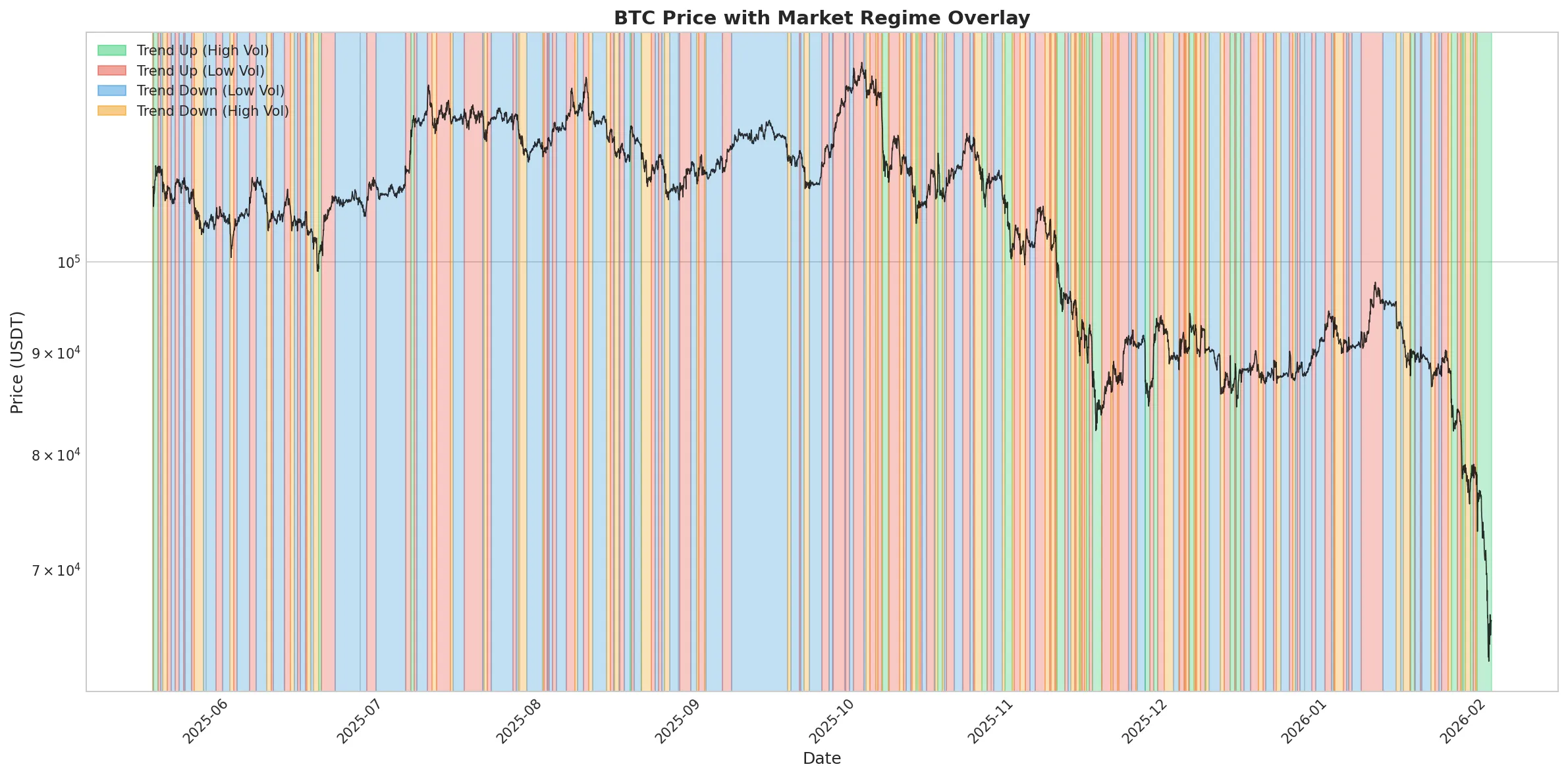
Figure 2: Transition matrix

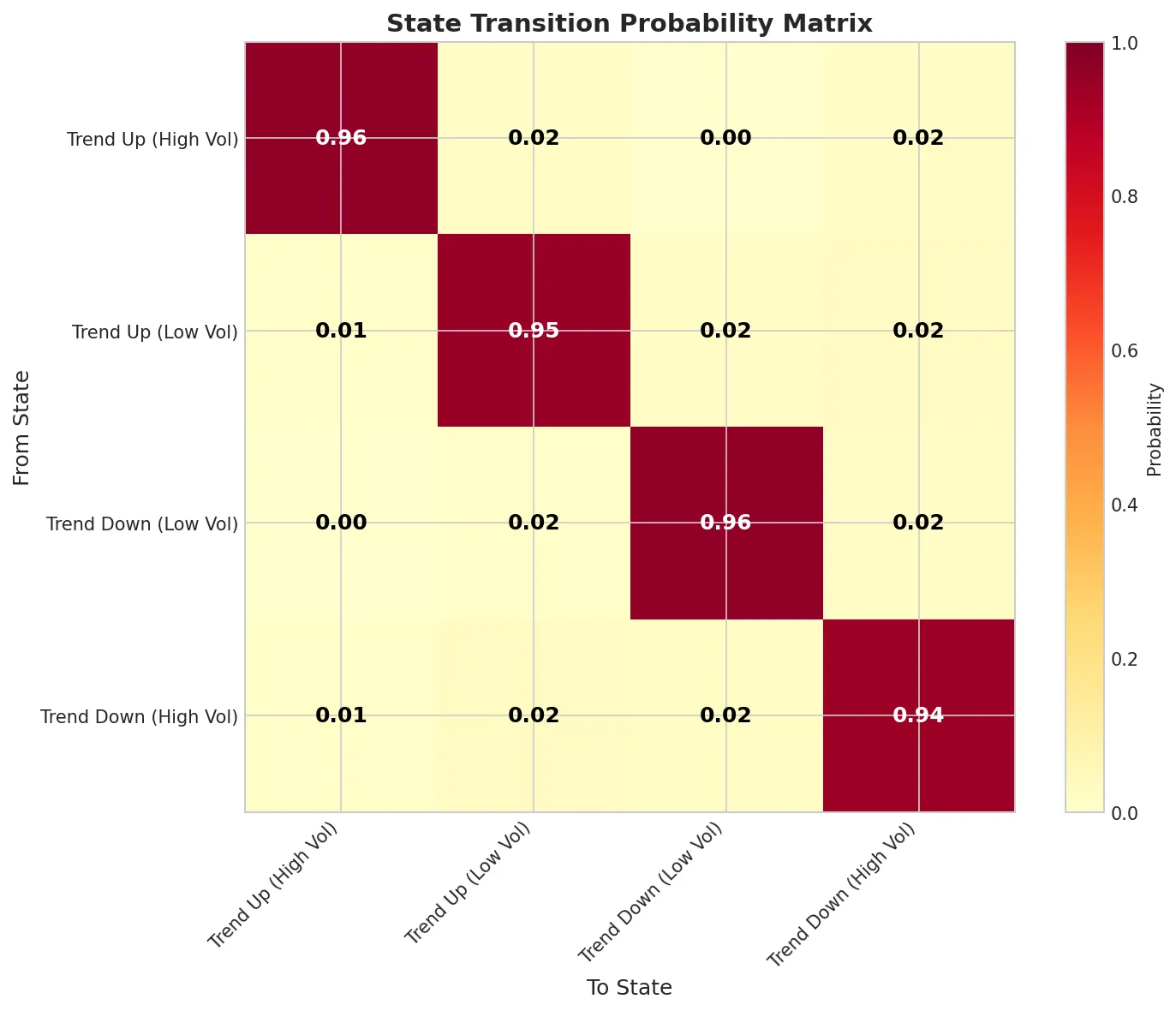
The transition matrix provides a direct probabilistic interpretation of regime stability and cross-regime movement intensity.

Closing Note

This project is still ongoing, and the model is not perfect at detecting market regimes yet. Still, I decided to share findings from my research on how HMM can be applied to market regime learning, especially for BTC where regime shifts and distribution tails are central to risk and strategy design.